The Linear Regression Estimator and Matrix Algebra

Estimation, Model Fit, and Matrix Algebra

Guidance for Midterm Exam

All material (lectures, readings, examples, etc.) are fair game for the exam.
I do not expect you to entirely reproduce proofs of theorems, but I expect you to recognize and understand the key ideas and be able to apply them.
You may be asked to elaborate on particular points and provide additional context or examples.
This may entail working through particular characteristics of the estimator – e.g., demonstrate the unbiasedness of the OLS estimator.

Guidance for Midterm Exam

Key terms and concepts: Normal equations, OLS estimator, Gauss-Markov theorem, OLS estimator, OLS residuals, etc.
Conceptual applications are common (e.g., what are the assumptions of the Gauss-Markov theorem? What does it tell us about the OLS estimator? How does it help us understand the OLS estimator?)
Interpretation is also important (e.g., what does the OLS estimator tell us about the relationship between \(X\) and \(Y\)?)

Example

Gauss-Markov Assumptions. If the PRF is written as: \(Y_i=\alpha+\beta X_i+\epsilon_i\), and the SRF is expressed as: \(Y_i=a+b X_i+e_i\).

What assumptions are required in order for the OLS estimator to be the best linear unbiased estimator with minimum variance? Describe each assumption in no more than 1-2 sentences.
The Gauss-Markov theorem holds that if these assumptions are met, the OLS estimator of \(b\) is a linear function of \(y_i\) (i.e., \(b=\sum k_i Y_i\)). Please demonstrate this.
The Gauss-Markov theorem holds that if these assumptions are met, the OLS estimator is an unbiased estimator of \(\beta\). Please demonstrate this (hint: use \(b=\sum k_i Y_i\) to show this is the case).

Part I: Estimation in R

The Data Generating Process (DGP)

The DGP is the underlying process that produces the sample data we observe — the PRF that generates the data.

Its the mechanism – we assume – generated the observed data + sampling error.

We can simulate data from a known DGP to understand how sampling, estimation, and inference work together.

Using a function in R

simulate_regression_data <- function(
  n = 500, beta_0 = 0, beta_1 = 0.2,
  x_mean = 0, x_sd = 1, error_sd = 1
) {
  X <- rnorm(n, mean = x_mean, sd = x_sd)
  errors <- rnorm(n, mean = 0, sd = error_sd)
  Y <- beta_0 + beta_1 * X + errors
  data.frame(x = X, y = Y, true_y = beta_0 + beta_1 * X, error = errors)
}

PRF vs. SRF: Visualizing the DGP

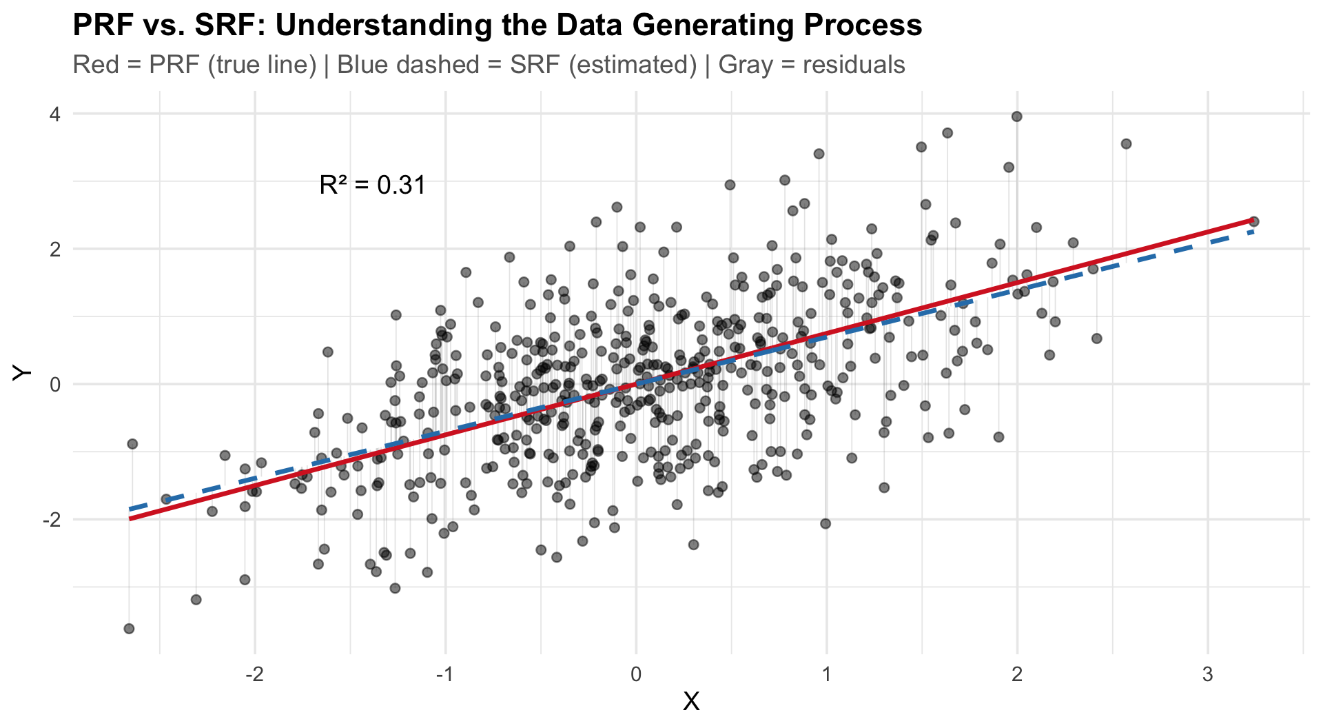
Key elements of the plot:

PRF (red solid): \(Y_i = \alpha + \beta X_i + \epsilon_i\) — the true line we never see
SRF (blue dashed): \(Y_i = a + bX_i + e_i\) — our estimate from the sample
Residuals (gray): \(e_i = Y_i - \hat{Y}_i\)

The SRF approximates the PRF. How well depends on:

Sample size \(n\)
Error variance \(\sigma^2_\epsilon\)
Variance of \(X\)

Estimation with `lm()`

fit <- lm(y ~ x, data = sim_dat)
summary(fit)


Call:
lm(formula = y ~ x, data = sim_dat)

Residuals:
     Min       1Q   Median       3Q      Max 
-2.75568 -0.67016  0.01042  0.63073  2.73709 

Coefficients:
              Estimate Std. Error t value Pr(>|t|)    
(Intercept) -0.0004678  0.0452219   -0.01    0.992    
x            0.6960271  0.0465049   14.97   <2e-16 ***
---
Signif. codes:  0 '***' 0.001 '**' 0.01 '*' 0.05 '.' 0.1 ' ' 1

Residual standard error: 1.011 on 498 degrees of freedom
Multiple R-squared:  0.3103,    Adjusted R-squared:  0.3089 
F-statistic:   224 on 1 and 498 DF,  p-value: < 2.2e-16

Estimation with `lm()`

Key elements of the output:

Element	Meaning
Coefficients	Estimated \(a\), \(b\) with SEs, t-values, p-values
Residual SE	Average distance of observations from the regression line
\(R^2\)	Proportion of variance in \(Y\) explained by \(X\)
F-statistic	Tests whether the model beats the null (\(\bar{Y}\))

Generating Predictions

# Single
predict(fit, newdata = data.frame(x = 1))

        1 
0.6955593

# Multiple values
predict(fit, newdata = data.frame(x = seq(0.25, 0.35, by = 0.05)))

        1         2         3 
0.1735390 0.2083404 0.2431417

# all fitted values...
predict(fit) |> head()

          1           2           3           4           5           6 
-0.39057401 -0.16067754  1.08443545  0.04860798  0.08952000  1.19326394

Predictions are just \(\hat{Y}_i = a + bX_i\) evaluated at chosen \(X\) values.

Part II: Model Fit

Model Fit: \(R^2\), Correlation, & ANOVA

The correlation \(r\) equals the standardized slope in bivariate regression:

Regression Estimates


Call:
lm(formula = scale(y) ~ scale(x), data = sim_dat)

Residuals:
     Min       1Q   Median       3Q      Max 
-2.26700 -0.55132  0.00857  0.51888  2.25170 

Coefficients:
             Estimate Std. Error t value Pr(>|t|)    
(Intercept) 3.351e-17  3.718e-02    0.00        1    
scale(x)    5.570e-01  3.722e-02   14.97   <2e-16 ***
---
Signif. codes:  0 '***' 0.001 '**' 0.01 '*' 0.05 '.' 0.1 ' ' 1

Residual standard error: 0.8313 on 498 degrees of freedom
Multiple R-squared:  0.3103,    Adjusted R-squared:  0.3089 
F-statistic:   224 on 1 and 498 DF,  p-value: < 2.2e-16

[1] 0.5570035

\(b_{x} \approx 0.557\)

Correlation Estimates

[1] 0.5570035

\(r_{xy} \approx 0.557\)

Key relationships:

\(R^2 = r^2\) in bivariate regression
\(r = \sqrt{R^2} \times \text{sign}(\beta)\)
The correlation is the standardized regression coefficient

Decomposing the Variance (ANOVA)

\[TSS = RegSS + RSS\]

\[\sum(Y_i - \bar{Y})^2 = \sum(\hat{Y}_i - \bar{Y})^2 + \sum(Y_i - \hat{Y}_i)^2\]

Component	Formula	Meaning
TSS	\(\sum(Y_i - \bar{Y})^2\)	Total variation in \(Y\)
RegSS	\(\sum(\hat{Y}_i - \bar{Y})^2\)	Variation explained by the model
RSS	\(\sum(Y_i - \hat{Y}_i)^2\)	Unexplained (residual) variation

\(R^2\): The Coefficient of Determination

\[R^2 = \frac{RegSS}{TSS} = 1 - \frac{RSS}{TSS}\]

\(R^2 = 0\): model explains nothing; \(E(Y|X) = \bar{Y}\)
\(R^2 = 1\): deterministic relationship; all points on the line

Proportional reduction in error — how much better is our model than just predicting \(\bar{Y}\)?

The F-statistic

\[F = \frac{RegSS / df_{reg}}{RSS / df_{res}} = \frac{MSS_{reg}}{MSS_{res}}\]

Where \(df_{reg} = k\) and \(df_{res} = n - k - 1\).

Hypotheses:

\(H_0\): \(\beta = 0\) (model no better than null)
\(H_a\): \(\beta \neq 0\) (model explains variance)

The F-statistic is a ratio of two variances — it follows the F-distribution under \(H_0\).

What Happens When You Vary Parameters?

Increase error (\(\sigma_\epsilon\)):

Points scatter more around PRF
\(R^2\) drops
Sampling distribution of \(b\) widens
But \(b\) remains unbiased

Increase \(\sigma_X\):

More spread in \(X\) → more leverage
\(R^2\) increases
\(var(b)\) decreases — more efficient

Increase \(n\):

SRF → PRF
Standard errors shrink \(\propto 1/\sqrt{n}\)
\(R^2\) stabilizes

Set \(\beta = 0\):

SRF still estimates some slope (sampling error)
Monte Carlo distribution centers on zero
This is the null hypothesis in action

Characteristics of the OLS Estimator

Part II: Matrix Algebra

Vectors, Matrices, and the OLS Estimator

Why Matrix Algebra?

Writing the SRF in matrix form makes it easier to solve
Quantitative social science aims to quantify relationships between multiple variables
Data is tabular: rows = observations, columns = variables
We need tools to solve systems of equations efficiently

\[\begin{bmatrix} y_{1}= & b_0+ b_1 x_{1}+b_2 x_{2}\\ y_{2}= & b_0+ b_1 x_{1}+b_2 x_{2}\\ \vdots\\ y_{n}= & b_0+ b_1 x_{1}+b_2 x_{2} \end{bmatrix}\]

\(n\) equations, fewer unknowns — linear algebra gives us the solution

Data as a Matrix

Each row is an observation; each column is a variable.

\[\begin{bmatrix} Vote & PID & Ideology \\\hline a_{11} & a_{12} & a_{13} \\ a_{21} & a_{22} & a_{23} \\ \vdots & \vdots & \vdots\\ a_{n1} & a_{n2} & a_{n3} \end{bmatrix}\]

This is an \(n \times 3\) matrix
First subscript = row, second = column
Notation: \(\mathbf{A}_{n \times 3}\)

A <- matrix(c(1, 0, 3,
              0, 1, 5,
              1, 1, 4), nrow = 3, byrow = TRUE)
colnames(A) <- c("Vote", "PID", "Ideology")
A

     Vote PID Ideology
[1,]    1   0        3
[2,]    0   1        5
[3,]    1   1        4

dim(A)

[1] 3 3

Vectors: The Building Blocks

Scalar: a single number (magnitude only)
Vector: multiple elements — encodes magnitude and direction

A vector \(\mathbf{a} \in \mathbb{R}^k\) has \(k\) elements.

Euclidean Distance between \(\mathbf{a}=[x_1,y_1]\) and \(\mathbf{b}=[x_2,y_2]\):

\[\text{Distance}(\mathbf{a},\mathbf{b}) = \sqrt{(x_1-x_2)^2+(y_1-y_2)^2}\]

This is just the Pythagorean theorem!

a <- c(3, 2); b <- c(1, 1)
sqrt(sum((a - b)^2))  # Euclidean distance

[1] 2.236068

The Norm of a Vector

The norm measures the length (magnitude) of a vector from the origin:

\[\|\mathbf{a}\| = \sqrt{x_1^2 + y_1^2}\]

Dividing a vector by its norm gives a unit vector (length = 1)
Useful for standardization

a <- c(3, 2, 1)
sqrt(sum(a^2))       # norm of a

[1] 3.741657

a / sqrt(sum(a^2))   # unit vector

[1] 0.8017837 0.5345225 0.2672612

In higher dimensions (\(\mathbb{R}^3\)):

\[\|\mathbf{a}\| = \sqrt{x_1^2 + y_1^2 + z_1^2}\]

Vector Addition & Subtraction

Element-wise operations on conformable vectors (same length):

\[\mathbf{a} + \mathbf{b} = [3+1,\; 2+1,\; 1+1] = [4, 3, 2]\]

\[\mathbf{a} - \mathbf{b} = [3-1,\; 2-1,\; 1-1] = [2, 1, 0]\]

Properties:

Property	Statement
Commutative	\(\mathbf{a}+\mathbf{b}=\mathbf{b}+\mathbf{a}\)
Associative	\((\mathbf{a}+\mathbf{b})+\mathbf{c}=\mathbf{a}+(\mathbf{b}+\mathbf{c})\)
Distributive	\(c(\mathbf{a}+\mathbf{b})=c\mathbf{a}+c\mathbf{b}\)
Zero	\(\mathbf{a}+0=\mathbf{a}\)

a <- c(3, 2, 1); b <- c(1, 1, 1)
a + b    # addition

[1] 4 3 2

a - b    # subtraction

[1] 2 1 0

Vector Multiplication

Inner (dot) product → produces a scalar (measures similarity / covariance)
Cross product → produces a vector (orthogonal to both inputs)
Outer product → produces a matrix

The Inner (Dot) Product

Multiply corresponding elements and sum:

\[\mathbf{a} \cdot \mathbf{b} = \sum_i a_i b_i\]

For \(\mathbf{a}=[3,2,1]\) and \(\mathbf{b}=[1,1,1]\): \(\;\; 3(1)+2(1)+1(1) = 6\)

a <- c(3, 2, 1); b <- c(1, 1, 1)
sum(a * b)          # inner product

[1] 6

a %*% b             # same thing with matrix notation

     [,1]
[1,]    6

The inner product is a measure of covariance:

\[\text{cov}(x,y) = \frac{\text{inner product}(x-\bar{x},\; y-\bar{y})}{n-1}\]

\[r_{x,y} = \frac{\text{inner product}(x-\bar{x},\; y-\bar{y})}{\|x-\bar{x}\|\;\|y-\bar{y}\|}\]

Inner Product Rules

Property	Statement
Commutative	\(\mathbf{a} \cdot \mathbf{b} = \mathbf{b} \cdot \mathbf{a}\)
Associative	\(d(\mathbf{a} \cdot \mathbf{b}) = (d\mathbf{a}) \cdot \mathbf{b}\)
Distributive	\(\mathbf{c} \cdot (\mathbf{a}+\mathbf{b}) = \mathbf{c}\cdot\mathbf{a} + \mathbf{c}\cdot\mathbf{b}\)
Zero	\(\mathbf{a} \cdot 0 = 0\)

The Cross Product

For \(\mathbf{a}=[3,2,1]\) and \(\mathbf{b}=[1,4,7]\):

Stack the vectors
Calculate \(2 \times 2\) determinants

\[\mathbf{a} \times \mathbf{b} = [2(7)-4(1),\;\; 1(1)-3(7),\;\; 3(4)-2(1)] = [10, -20, 10]\]

Result is orthogonal to both original vectors
Useful for determinants and matrix inversion

The Outer Product

Transpose one vector, then multiply:

\[\begin{bmatrix} 3 \\ 2 \\ 1 \end{bmatrix} \begin{bmatrix} 1 & 4 & 7 \end{bmatrix} = \begin{bmatrix} 3 & 12 & 21 \\ 2 & 8 & 14 \\ 1 & 4 & 7 \end{bmatrix}\]

Input: two vectors of length \(k\)
Output: a \(k \times k\) matrix

a <- c(3, 2, 1); b <- c(1, 4, 7)
a %o% b   # outer product

     [,1] [,2] [,3]
[1,]    3   12   21
[2,]    2    8   14
[3,]    1    4    7

Matrices

A matrix combines row or column vectors. Notation: bold uppercase (\(\mathbf{A}\)).

\[\begin{bmatrix} a_{11} & a_{12} & \cdots & a_{1n} \\ a_{21} & a_{22} & \cdots & a_{2n} \\ \vdots & \vdots & \ddots & \vdots\\ a_{n1} & a_{n2} & \cdots & a_{nn} \end{bmatrix}\]

Matrix Types

Type	Definition
Square	Equal rows and columns
Symmetric	Same entries above and below the diagonal; \(\mathbf{A} = \mathbf{A}^T\)
Identity (\(\mathbf{I}\))	1s on diagonal, 0s off; \(\mathbf{AI} = \mathbf{A}\)
Idempotent	\(\mathbf{A}^2 = \mathbf{A}\)
Trace	Sum of diagonal elements: \(\text{tr}(\mathbf{I}) = n\)

Matrix Addition & Subtraction

Matrices must be conformable (same dimensions). Add/subtract element-wise:

\[\begin{bmatrix} a_{11} & a_{12} \\ a_{21} & a_{22} \end{bmatrix} + \begin{bmatrix} b_{11} & b_{12} \\ b_{21} & b_{22} \end{bmatrix} = \begin{bmatrix} a_{11}+b_{11} & a_{12}+b_{12} \\ a_{21}+b_{21} & a_{22}+b_{22} \end{bmatrix}\]

Properties: Commutative, Associative, Distributive, Zero

Matrix Multiplication

Order matters! \(\mathbf{AB} \neq \mathbf{BA}\) in general.

Multiply \(i\)-th row by \(j\)-th column:

\[\begin{bmatrix} 1 & 3 \\ 2 & 4 \end{bmatrix} \begin{bmatrix} 3 & 5 \\ 2 & 4 \end{bmatrix} = \begin{bmatrix} 1(3)+3(2) & 1(5)+3(4) \\ 2(3)+4(2) & 2(5)+4(4) \end{bmatrix} = \begin{bmatrix} 9 & 17 \\ 14 & 26 \end{bmatrix}\]

A <- matrix(c(1,3,2,4), nrow=2, byrow=TRUE)
B <- matrix(c(3,5,2,4), nrow=2, byrow=TRUE)
A %*% B

     [,1] [,2]
[1,]    9   17
[2,]   14   26

Conformability rule: columns of first = rows of second

\[\mathbf{A}_{m \times n} \times \mathbf{B}_{n \times p} = \mathbf{C}_{m \times p}\]

Inner dimensions must match; result has outer dimensions.

The Transpose

\(\mathbf{A}^T\) swaps rows and columns. If \(\mathbf{A}\) is \(m \times n\), then \(\mathbf{A}^T\) is \(n \times m\).

\[\begin{bmatrix} 1 & 2 & 3 \\ 4 & 5 & 6 \end{bmatrix}^T = \begin{bmatrix} 1 & 4 \\ 2 & 5 \\ 3 & 6 \end{bmatrix}\]

A <- matrix(c(1,2,3,4,5,6), nrow=2, byrow=TRUE)
t(A)         # transpose

     [,1] [,2]
[1,]    1    4
[2,]    2    5
[3,]    3    6

t(A) %*% A   # A'A is always square & symmetric

     [,1] [,2] [,3]
[1,]   17   22   27
[2,]   22   29   36
[3,]   27   36   45

Key properties:

Property	Statement
Double transpose	\((\mathbf{A}^T)^T = \mathbf{A}\)
Sum	\((\mathbf{A}+\mathbf{B})^T = \mathbf{A}^T + \mathbf{B}^T\)
Product (reversal)	\((\mathbf{AB})^T = \mathbf{B}^T\mathbf{A}^T\)

Why the Transpose Matters

Transposing a product reverses the order:

\[(\mathbf{ABC})^T = \mathbf{C}^T\mathbf{B}^T\mathbf{A}^T\]

Critical result: For any matrix \(\mathbf{A}\), the product \(\mathbf{A}^T\mathbf{A}\) is always:

Square (\(n \times n\) if \(\mathbf{A}\) is \(m \times n\))
Symmetric

This is exactly what \(\mathbf{X}^T\mathbf{X}\) produces in the normal equations.

The Determinant

The determinant is a scalar value computed from a square matrix. It’s necessary for matrix inversion (later).

For a \(2 \times 2\) matrix:

\[\det(\mathbf{A}) = \det\begin{bmatrix} a & b \\ c & d \end{bmatrix} = ad - bc\]

If \(\det(\mathbf{A}) \neq 0\): the matrix is nonsingular (invertible)
If \(\det(\mathbf{A}) = 0\): the matrix is singular (no inverse exists — columns are linearly dependent)

Example:

\[\det\begin{bmatrix} 4 & 7 \\ 2 & 6 \end{bmatrix} = 4(6) - 7(2) = 10 \neq 0 \;\; ✓\]

\[\det\begin{bmatrix} 2 & 4 \\ 1 & 2 \end{bmatrix} = 2(2) - 4(1) = 0 \;\; \text{(singular — row 1 = 2 × row 2)}\]

A <- matrix(c(4,7,2,6), nrow=2, byrow=TRUE)
det(A)   # nonsingular

[1] 10

B <- matrix(c(2,4,1,2), nrow=2, byrow=TRUE)
det(B)   # singular — no inverse

[1] 0

For OLS: \(\det(\mathbf{X}^T\mathbf{X}) = 0\) means perfect multicollinearity — the columns of \(\mathbf{X}\) are linearly dependent, and we cannot solve for \(\mathbf{b}\).

Matrix Inversion

For scalars: \(a \cdot a^{-1} = 1\)

For matrices: \(\mathbf{A}\mathbf{A}^{-1} = \mathbf{A}^{-1}\mathbf{A} = \mathbf{I}\)

Requirements:

Only square matrices can have inverses
Must be nonsingular: \(\det(\mathbf{A}) \neq 0\)

The \(2 \times 2\) Inverse

\[\mathbf{A} = \begin{bmatrix} a & b \\ c & d \end{bmatrix} \quad \Longrightarrow \quad \mathbf{A}^{-1} = \frac{1}{ad-bc}\begin{bmatrix} d & -b \\ -c & a \end{bmatrix}\]

Example:

\[\begin{bmatrix} 4 & 7 \\ 2 & 6 \end{bmatrix}^{-1} = \frac{1}{10}\begin{bmatrix} 6 & -7 \\ -2 & 4 \end{bmatrix} = \begin{bmatrix} 0.6 & -0.7 \\ -0.2 & 0.4 \end{bmatrix}\]

\[\mathbf{A}\mathbf{A}^{-1} = \begin{bmatrix} 1 & 0 \\ 0 & 1 \end{bmatrix} = \mathbf{I} \;\; ✓\]

A <- matrix(c(4,7,2,6), nrow=2, byrow=TRUE)
solve(A)          # inverse

     [,1] [,2]
[1,]  0.6 -0.7
[2,] -0.2  0.4

A %*% solve(A)    # verify: should be identity

              [,1]          [,2]
[1,]  1.000000e+00 -1.110223e-16
[2,] -1.110223e-16  1.000000e+00

Properties of the Inverse

Property	Statement
Product (reversal)	\((\mathbf{AB})^{-1} = \mathbf{B}^{-1}\mathbf{A}^{-1}\)
Transpose	\((\mathbf{A}^T)^{-1} = (\mathbf{A}^{-1})^T\)
Double inverse	\((\mathbf{A}^{-1})^{-1} = \mathbf{A}\)
Identity	\(\mathbf{I}^{-1} = \mathbf{I}\)

Like the transpose, inverting a product reverses the order.

Linear Regression in Matrix Form

\[\mathbf{y} = \mathbf{X}\mathbf{b} + \mathbf{e}\]

\[\mathbf{y} = \begin{bmatrix} Y_1 \\ Y_2 \\ \vdots \\ Y_n \end{bmatrix} \quad \mathbf{b} = \begin{bmatrix} b_0 \\ b_1 \\ \vdots \\ b_k \end{bmatrix}\]

\[\mathbf{X} = \begin{bmatrix} 1 & X_{11} & \cdots & X_{1k} \\ 1 & X_{21} & \cdots & X_{2k} \\ \vdots & \vdots & \ddots & \vdots \\ 1 & X_{n1} & \cdots & X_{nk} \end{bmatrix}\]

Deriving the OLS Estimator

Same Objective: Minimize the sum of squared errors. In scalar form, we minimized \(\sum e_i^2\). In matrix form:

\[\min_{\mathbf{b}}\; \mathbf{e}^T\mathbf{e} = (\mathbf{y} - \mathbf{Xb})^T(\mathbf{y} - \mathbf{Xb})\]

Expand using the distributive property of the transpose, \((\mathbf{A} - \mathbf{B})^T = \mathbf{A}^T - \mathbf{B}^T\):

\[\mathbf{e}^T\mathbf{e} = (\mathbf{y}^T - \mathbf{b}^T\mathbf{X}^T)(\mathbf{y} - \mathbf{Xb})\]

Multiply out the terms:

\[= \mathbf{y}^T\mathbf{y} - \mathbf{y}^T\mathbf{Xb} - \mathbf{b}^T\mathbf{X}^T\mathbf{y} + \mathbf{b}^T\mathbf{X}^T\mathbf{X}\mathbf{b}\]

The middle two terms are both scalars (a \(1 \times 1\) result), and a scalar equals its own transpose: \(\mathbf{y}^T\mathbf{Xb} = (\mathbf{b}^T\mathbf{X}^T\mathbf{y})^T = \mathbf{b}^T\mathbf{X}^T\mathbf{y}\). So they combine:

\[\mathbf{e}^T\mathbf{e} = \mathbf{y}^T\mathbf{y} - 2\mathbf{b}^T\mathbf{X}^T\mathbf{y} + \mathbf{b}^T\mathbf{X}^T\mathbf{X}\mathbf{b}\]

Taking the Derivative: What Does It Mean?

In scalar calculus, \(\frac{d}{db} f(b)\) gives a single number. In matrix calculus, \(\frac{\partial f}{\partial \mathbf{b}}\) gives a vector of partial derivatives — one for each element of \(\mathbf{b}\).

If \(\mathbf{b} = [b_0, b_1, \ldots, b_k]^T\), then:

\[\frac{\partial f}{\partial \mathbf{b}} = \begin{bmatrix} \frac{\partial f}{\partial b_0} \\ \frac{\partial f}{\partial b_1} \\ \vdots \\ \frac{\partial f}{\partial b_k} \end{bmatrix}\]

This vector of partial derivatives is the gradient — it points in the direction of steepest ascent. Setting it to \(\mathbf{0}\) means every partial derivative equals zero simultaneously.

The Jacobian

The Jacobian generalizes the derivative to vector-valued functions. If a function maps \(k\) inputs to \(m\) outputs, the Jacobian is the \(m \times k\) matrix of all partial derivatives:

\[\mathbf{J} = \begin{bmatrix} \frac{\partial f_1}{\partial b_0} & \frac{\partial f_1}{\partial b_1} & \cdots & \frac{\partial f_1}{\partial b_k} \\ \frac{\partial f_2}{\partial b_0} & \frac{\partial f_2}{\partial b_1} & \cdots & \frac{\partial f_2}{\partial b_k} \\ \vdots & \vdots & \ddots & \vdots \\ \frac{\partial f_m}{\partial b_0} & \frac{\partial f_m}{\partial b_1} & \cdots & \frac{\partial f_m}{\partial b_k} \end{bmatrix}\]

For OLS, our function \(f(\mathbf{b}) = \mathbf{e}^T\mathbf{e}\) is scalar-valued (\(m = 1\)), so the Jacobian is a single row — which is just the transpose of the gradient:

\[\mathbf{J} = \left[\frac{\partial f}{\partial b_0}, \;\frac{\partial f}{\partial b_1}, \;\ldots,\; \frac{\partial f}{\partial b_k}\right]\]

Why does this matter? In the bivariate case, we took two separate derivatives (\(\frac{\partial SSR}{\partial a}\) and \(\frac{\partial SSR}{\partial b}\)) and solved two equations. The gradient/Jacobian does the same thing — but for all \(k+1\) coefficients at once, packaged as a single matrix operation. This is why matrix notation is powerful: one equation replaces \(k+1\) equations.

Matrix Derivative Rules

We need three rules — each mirrors scalar calculus:

Scalar Rule	Matrix Rule
\(\frac{d}{db}(c) = 0\)	\(\frac{\partial}{\partial \mathbf{b}}(\mathbf{y}^T\mathbf{y}) = \mathbf{0}\)
\(\frac{d}{db}(\mathbf{c}^T b) = \mathbf{c}\)	\(\frac{\partial}{\partial \mathbf{b}}(\mathbf{c}^T\mathbf{b}) = \mathbf{c}\)
\(\frac{d}{db}(b^2 a) = 2ab\)	\(\frac{\partial}{\partial \mathbf{b}}(\mathbf{b}^T\mathbf{A}\mathbf{b}) = 2\mathbf{A}\mathbf{b}\) (if \(\mathbf{A}\) is symmetric)

The third rule requires \(\mathbf{A}\) to be symmetric. Since \(\mathbf{X}^T\mathbf{X}\) is always symmetric (recall: \((\mathbf{X}^T\mathbf{X})^T = \mathbf{X}^T\mathbf{X}\)), the rule applies.

Applying the Rules

Our function is: \(\;\mathbf{e}^T\mathbf{e} = \underbrace{\mathbf{y}^T\mathbf{y}}_{\text{constant}} - \underbrace{2\mathbf{b}^T\mathbf{X}^T\mathbf{y}}_{\text{linear in } \mathbf{b}} + \underbrace{\mathbf{b}^T\mathbf{X}^T\mathbf{X}\mathbf{b}}_{\text{quadratic in } \mathbf{b}}\)

Term by term:

Term	Rule Applied	Derivative w.r.t. \(\mathbf{b}\)
\(\mathbf{y}^T\mathbf{y}\)	Constant → 0	\(\mathbf{0}\)
\(-2\mathbf{b}^T\mathbf{X}^T\mathbf{y}\)	Linear: \(\frac{\partial}{\partial \mathbf{b}}(\mathbf{c}^T\mathbf{b}) = \mathbf{c}\), where \(\mathbf{c} = \mathbf{X}^T\mathbf{y}\)	\(-2\mathbf{X}^T\mathbf{y}\)
\(\mathbf{b}^T\mathbf{X}^T\mathbf{X}\mathbf{b}\)	Quadratic: \(\frac{\partial}{\partial \mathbf{b}}(\mathbf{b}^T\mathbf{A}\mathbf{b}) = 2\mathbf{A}\mathbf{b}\), where \(\mathbf{A} = \mathbf{X}^T\mathbf{X}\)	\(2\mathbf{X}^T\mathbf{X}\mathbf{b}\)

Combining: \(\;\frac{\partial\; \mathbf{e}^T\mathbf{e}}{\partial\; \mathbf{b}} = -2\mathbf{X}^T\mathbf{y} + 2\mathbf{X}^T\mathbf{X}\mathbf{b}\)

Setting the Derivative to Zero

Combining the terms:

\[\frac{\partial\; \mathbf{e}^T\mathbf{e}}{\partial\; \mathbf{b}} = -2\mathbf{X}^T\mathbf{y} + 2\mathbf{X}^T\mathbf{X}\mathbf{b} = 0\]

Rearrange (move \(-2\mathbf{X}^T\mathbf{y}\) to the right, divide by 2):

\[\mathbf{X}^T\mathbf{X}\mathbf{b} = \mathbf{X}^T\mathbf{y}\]

These are the normal equations — the matrix version of the first-order conditions.

Solve for \(\mathbf{b}\) by multiplying both sides on the left by \((\mathbf{X}^T\mathbf{X})^{-1}\):

\[(\mathbf{X}^T\mathbf{X})^{-1}\mathbf{X}^T\mathbf{X}\mathbf{b} = (\mathbf{X}^T\mathbf{X})^{-1}\mathbf{X}^T\mathbf{y}\]

Since \((\mathbf{X}^T\mathbf{X})^{-1}\mathbf{X}^T\mathbf{X} = \mathbf{I}\) and \(\mathbf{Ib} = \mathbf{b}\):

\[\boxed{\mathbf{b} = (\mathbf{X}^T\mathbf{X})^{-1}\mathbf{X}^T\mathbf{y}}\]

This requires \(\mathbf{X}^T\mathbf{X}\) to be invertible — fails under perfect multicollinearity.

x <- c(1, 2, 3, 4, 5)
y <- c(5.1, 7.9, 11.2, 13.8, 17.1)
X <- cbind(1, x)    
b <- solve(t(X) %*% X) %*% t(X) %*% y
b                    # OLS

  [,1]
  2.05
x 2.99

coef(lm(y ~ x))     # verify with lm()

(Intercept)           x 
       2.05        2.99

Summary

Vectors encode magnitude and direction; the inner product measures covariance
Matrices combine vectors; operations require conformability
Transpose swaps rows/columns; transposing a product reverses order
Inversion is the matrix analog of division; requires a nonsingular matrix
The OLS estimator in matrix form: \(\mathbf{b} = (\mathbf{X}^T\mathbf{X})^{-1}\mathbf{X}^T\mathbf{y}\)

References

Gill, Jeff. 2006. Essential Mathematics for Political and Social Research. Cambridge.
Moore, Will and David Siegel. 2013. A Mathematics Course for Political and Social Research. Princeton.

The Linear Regression Estimator and Matrix Algebra

Guidance for Midterm Exam

Guidance for Midterm Exam

Example

Part I: Estimation in R

The Data Generating Process (DGP)

PRF vs. SRF: Visualizing the DGP

Key elements of the plot:

Estimation with lm()

Estimation with lm()

Generating Predictions

Part II: Model Fit

Model Fit: \(R^2\), Correlation, & ANOVA

Correlation Estimates

Decomposing the Variance (ANOVA)

\(R^2\): The Coefficient of Determination

The F-statistic

What Happens When You Vary Parameters?

Characteristics of the OLS Estimator

Part II: Matrix Algebra

Why Matrix Algebra?

Data as a Matrix

Vectors: The Building Blocks

The Norm of a Vector

Vector Addition & Subtraction

Vector Multiplication

The Inner (Dot) Product

Inner Product Rules

The Cross Product

The Outer Product

Matrices

Matrix Types

Matrix Addition & Subtraction

Matrix Multiplication

The Transpose

Why the Transpose Matters

The Determinant

Matrix Inversion

The \(2 \times 2\) Inverse

Properties of the Inverse

Linear Regression in Matrix Form

Deriving the OLS Estimator

Taking the Derivative: What Does It Mean?

The Jacobian

Matrix Derivative Rules

Applying the Rules

Setting the Derivative to Zero

Summary

References

Estimation with `lm()`

Estimation with `lm()`